Concrete Bridge Design Workflow

The last few months I’ve been working intensively on a complete workflow for detailed design of concrete bridges with Autodesk Revit. In case you would ask me “Is Revit even capable of designing bridges with a high level of detail?” Well, my answer would be “Definitely YES !” And I would like to share you the results in what is probably my longest post ever on this blog. So take your time to read it…

Introduction

Before I start explaining, maybe some background first. Some months ago, I needed to develop a POC of bridge design with Revit for some important customer meetings. In the past you might have seen already a solution from my colleague at Autodesk, Matthias Stark, which he explained in this class at AU 2015. Also Simon Moreau, author of the BIM42 blog based himself on this method in this post. So first of all, thank you Matthias and Simon for the inspiration. The workflow below is a consolidation of Matthias his method and the method I already used previously. The result is an easy to use flow, applicable on any type of concrete deck or box bridges or even concrete tunnels, using some Dynamo scripts that I have predefined for your personal use. All the data referred to can be downloaded at the bottom of this post.

Workflows

The full workflow from conceptual road/bridge design until detailed bridge design consists of 16 steps, which are all explained in this YouTube playlist “Concrete Bridge Design to Fabrication Workflow”. The image below shows a global overview on this workflow. This is a representation of what is possible currently possible with our solutions at Autodesk, and shows a positioning of the products for each phase.

1. The conceptual road and bridge design can be done using Infraworks 360.
2. This Infraworks model is then imported in AutoCAD Civil 3D for further detailing of the road design.
3. The data, built up in AutoCAD Civil 3D, is then reused in Revit and Dynamo (by means of Feature Lines, Corridor Points reports, …) to get the detailed bridge design.
4. Finally the bridge rebar detailing and design documentation are further processed in Revit.

This workflow is also setting the base for extended construction workflows. As all the concrete bridge design data is stored in the Revit model, it can be used in Construction Management (sequencing, quantification, clash detection) and Project Delivery Management. This involves BIM360 Glue, BIM360 Field, Navisworks Manage, BIM360 Docs,… An overview of the possible workflows can be found in the Bridge Design to Fabrication Workflows.pdf file which is included in the datasets at the bottom of this post.

So, this post is limited to the design steps with the creation of the superstructure deck family and the distribution of transversal rebar in the deck.

BRIDGE SUPERSTRUCTURE CREATION

Before building this family, I listed up some requirements which the bridge deck family should meet.

• The superelevation, width and thus also the slope for each lane are calculated from the Civil 3D data.
• The family needs to be flexible and modifiable afterwards in the Revit project.
• The Dynamo script used for the creation should be as small as possible and should be generic to use with other bridge sections or even tunnels.
• The family should be built up that way that it can host annotations in 2D Section views (even if the section goes through a curve).
• The family needs to be able to host rebar.
• The Dynamo script needs to be able to handle any orientation of a bridge (seen in a planview), in any position of a circle quadrant.

Meeting these requirements, this method differentiates from current methods existing already on the internet.

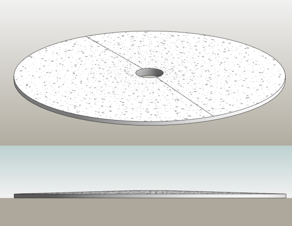
As you will see in this part of the playlist, the superstructure is created based on Civil 3D Corridor points and a Mass family representing the section profile of the deck. This “profile” is placed within the Revit main “Concrete Deck” family and then lofted to get a solid geometry.

Prerequisites

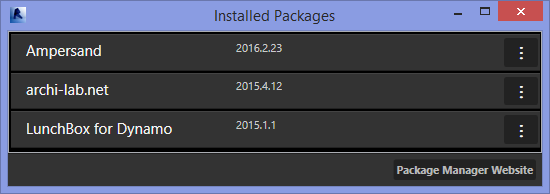
Before you start trying this yourself you need to install the package BIM4Struc.BridgeDesign through the Package Manager in Dynamo.

The Dynamo script “01 Bridge Superstructure Creation.dyn” used for this, is included in the datasets at the bottom of this post.

Step 1 – Extract Civil 3D Corridor Points

The geometry of the bridge deck should be based on the solid geometry of the road, which is designed in AutoCAD Civil 3D. Important is that the slopes of each lane of the road can vary along the road length (ie. from -2.5% to +2.5%). This information is extracted from Civil 3D using the “Corridor Points Report” and this data is stored in an Excel sheet. In this method it needs points for the Top Left, Top Right and Top Center edges of the road. Using Marker Points in Civil 3D you can give your own names to these points. This step is explained in this video.

Note: the reason why I used the Corridor Points Report and not just Feature Lines as an imported geometry in Dynamo, is explained in the reactions on this post (click on the balloon next the post title).

Step 2 – Create the section profile

As part of the “mise-en-place” you also need to create a family representing the section profile of the deck (T-deck, box girder or even tunnel). This is based on a “Metric Mass” family template. Make sure you create parameters for the superelevation, lane width and slope at the right and left of the road. As shown at 1:10 in this video, the values for the superelevation are recalculated within the family in order to handle positive and negative values.

After saving this family (“Concrete Deck Profile.rfa”), you load this one into a new family based on the “Metric Generic Model Adaptive.rft” template. You can change the behavior of this family in the Family Category & Parameters dialog. From there on we will use Dynamo to create the geometry.

Step 3 – Reading road data into Dynamo

Now we can start combining the information from step 1 and 2. This step starts at 2:11 in this video. The information about the road geometry can be read into Dynamo as a starter. The custom node “Road Splines from Excel” from the BIM4Struc.BridgeDesign package helps reading this Corridor Points report, by indicating the proper column indexes and Point Code descriptions (i.e. “RoadTopLeft”). If you choose to name these points differently in the Civil 3D model, then you need to change their descriptions as well in the Dynamo script.

In case the data changes in Civil 3D, you just need to regenerate the Corridor Points Report to Excel and rerun the script.
The result of this operation are 4 3D Polycurves representing the road top edges (left, right and center) and also the projection of the centerline at level 0 m. These lines will be used later to calulate the superelevations (lane slopes) at specific intervals.

The ConversionMultiplier can be used to convert the units. By default it is set to 1000 to convert the metric “m” used in the Civil 3D model to “mm”, which is the unit used in the Revit project.

Note that within the custom node, the coordinates are reset to the internal Revit origin, this to avoid the geometry being positioned at geographic coordinates in a Family. To achieve that, the coordinates of the start point of the centerline are set to 0, while the other coordinates are recalculated relatively to that point. Afterwards this will make it easier to position the bridge deck family in the Revit project (i.e. based on the imported feature lines in Revit).

Step 4 – Setting the bridge deck parameters in Dynamo

Before continuing with the geometry we need to setup the bridge parameters:

• Bridge Alignment Variables:
  This group allows to add an offset and/or skew angle to the first and last profile of the bridge deck. These values are further on used to divide the alignment lines.
• Bridge Superstructure Section Definition
  The configuration of this group depends on the way the “Concrete Deck Profile” family is created. In this optional part you can set the type parameters of the nested family, before it is placed.

Step 5 – Generating the bridge deck geometry with Dynamo

Starting at 3:25 in this video a second custom node is brought into the script. The node Bridge Section Profile Placement from the BIM4Struc.BridgeDesign package will place the initially created “Concrete Deck Profile” family at the right positions and orientation. The node is built in a way it doesn’t matter in which quadrant of a circle the planview of the bridge is positioned and orientated. It will adjust the profiles accordingly. Practically this means that the centerline points can have coordinates with syntaxis (-x,-y), (-x,y), (x,y) and (x,-y).

This custom node needs the Polycurves from the road and the centerline at level 0 m as inputs. The ProfilePositionParameters port needs a list with values between 0 and 1 indicating the positions of the profile. The more elements in the list, the more accurate the curvature of the horizontal alignment. But don’t exaggerate as this influences the number of section profile instances placed in the family (and thus makes it heavier). Next you also connect the proper family type (Concrete Deck Profile.rfa in this case) to the Profile input port. And the skew angles at start and end can be indicated as well.

The outputs of this node return the ProfileInstances placed in the Revit family as well as the generated points on each road edge in Dynamo. The ProfileInstances are used in Step 7, when we need to integrate the calculated values from Step 6 into the Revit family.

Important to know is that in this step only the position and orientation of the section profiles are handled. The results of the generated points (bottom 3 output ports) are further used in Step 6 to define the individual section dimensions.

Step 6 – Calculate dimensions of each section profile

Now we know the coordinates and orientation of each division point on the road edges in Dynamo, we can calculate the values of the superelevation and thus also the width and slope of each road lane. This is shown starting from 4:26 in this video.
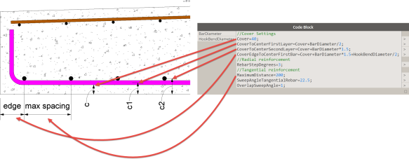
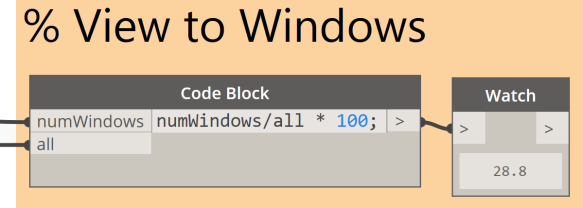
The procedure to calculate doesn’t need to be changed as long as you use the ‘three edge method’ to detect the road geometry. If your section profile uses different parameters names for  the Lane Width and Lane Slope, then off course you need to change their references in the Dynamo script in the middle Code Block shown in the image above.

Step 7 – Modify profile instances and create geometry

The results of the parameter calculations in Step 6 are connected with the Element.SetParameterByName node, and this will make the proper changes to each individual section profile placed in the Revit family. The geometry of the section profile instances is send back to Dynamo (Element.Curves) and used to create the solid deck geometry by means of the Form.ByLoftCrossSections node. Starting at 4:50 in this video.

I’ve decided not to group all these parameter calculation and solid creation nodes into a custom node, as it might happen that you use a different set of parameters, instances, … This way, the script is flexible for you to change if needed.

Step 8 – Flexible and modifiable family

The last section of this workflow (starting at 5:52 in this video) may be the most important one. After the Dynamo script has run and been closed, it is still possible to change the properties of the section profiles (in red) – which are by the way placed in a different subcategory for better visualization management in the project.

When you connect the instance parameters of the nested “Concrete Deck Profile” family with the family parameters of the main deck family, then you make it even possible to change the dimensions of the deck geometry from within the Revit project.

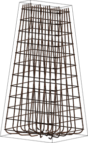
ADDING STRUCTURAL REBAR TO THE BRIDGE DECK

I think we all can agree that a concrete bridge deck geometry without reinforcement details added is like a pub without beer…

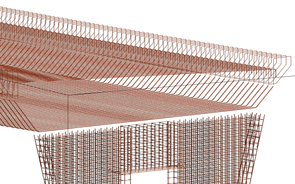
This part of the workflow will give you some insight in the possibilities that Dynamo offers to Revit when modelling complex rebar cages into the curved deck. There are many methods to achieve this, and there are also lots of varieties in the rebar shapes. The method described below is a generic usable one for the modelling of the transversal rebar cages, and is based on a “distribution along path” principle.
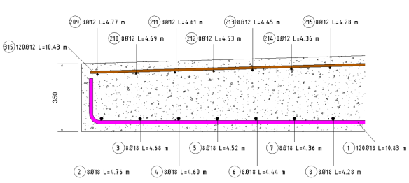
The results are shown in this video from the playlist. In the next steps, it is described how to get to this result.

Prerequisites

The method used here needs the BIM4Struc.Rebar and Dynamo for Rebar packages to be installed in Dynamo.

The Dynamo script “07 Transversal Rebar Distribution.dyn” used for this, is included in the datasets at the bottom of this post.

Step 1 – Model a base set of reinforcement

Before you start it is necessary to have modelled a base set of transversal reinforcement in the bridge deck. This can be done with the out-of-the-box Revit tools. This base set has the right properties already. Optionally you can save the rebar objects in a Selection Set in Revit, in order to find it back easily after distribution and to delete it then. (See 0:17 on this video)

Step 2 – Import the base rebar geometry in Dynamo

This base set of rebar objects will be used to generate a distributed set of rebar. Therefore we need to read the original geometry of the rebar elements into Dynamo. This is done in the “Get Rebar sketch from Revit” group, by means of the Rebar.GetCenterlineCurve node (from the BIM4Struc.Rebar package). The node returns the sketch behind the 3D Rebar object in Revit. (Read the input port tooltips on the node for more information about the options). The resulting curves can now be used to be distributed within the deck geometry. In the same time the Revit ID of the object hosting the base rebar is read too, to use it further in the Rebar creation step.

(From 0:25 on this video)

Step 3 – Define position and orientation of base rebar

This step is needed to detect the right orientation of the base rebar set and its relative position to the selected distribution path (Select Edge from Step 2). This information is crucial to make the distribution working. The position and orientation is represented then by the Curve.CoordinateSystemAtParameter node

Step 4 – Distribute the rebar sketch lines in Dynamo

The geometry from Step 2 combined with the position and orientation data from Step 3, results in a new list of geometry representing the equally distributed rebar sketch lines.

Step 5 – Create Rebar geometry in Revit

Finally (as seen at  0:59 on this video), the resulted curves are used to create the Rebar objects in Revit, with the Rebar.ByCurve node from the Dynamo for Rebar package To use the same properties for the newly created Rebar, the properties from the selected base set are read by the Rebar.GetProperties node from the BIM4Struc.Rebar package.

MORE DYNAMO FOR REBAR ?

The datasets below contain more scripts to create the longitudinal reinforcement i.e.

The described method above, together with some more “rebar awesomeness” will be presented and explained more in detail in this class at AU 2016 in Las Vegas, later this year.

DATASETS

The datasets used in this workflow can be downloaded here.

I hope you enjoyed reading and that this workflow may be of use for your daily work !

Rebar productivity tools for Revit with Dynamo

I finally started to gather all the custom nodes I have been creating for the creation of rebar objects in Revit using Dynamo. Besides using the Dynamo for Rebar package from CORE Studio, I also created some small productivity tools that can help you driving your rebar design. The package for Dynamo that has been published is called BIM4Struc.Rebar.

At this moment it consists of a limited number of custom nodes, but there will be added more and more, as AU gets nearer.

The ones that exist now in the package as a starter:

Rebar.GetHost returns the Revit ID of the host that contains the rebar object. In case that the rebar is not hosted, then it will be returned in the NonHostedRebar.

Rebar.GetCenterlineCurve is a node that returns the sketch geometry of a rebar, which is in fact the centerline. This is very handy when distributing existing complex rebars along 3D curves (using the Dynamo for Rebar package again).

Rebar.GetProperties is a node that extracts all necessary rebar properties from a selected rebar in Revit. These properties can be used in combination with the Dynamo for Rebar creation nodes to copy existing rebar for instance.

This helped me to make a quite short script to build the rebar in this double curved deck.

There will be explained more on this in future blog posts !

See keep an eye on it !

Clearance Height on Stairs – Watch your head!

The ergonomics of a stair is not only about the tread depth, the riser height, the stair slope, … It is also about the safety of your head when you walk the stair. Ever been in a situation when you rushed down the stair to the cellar and then bumped your head against one of the floor beams 😉

In this post I will explain you how to create your own Dynamo script for the “Clearance Height Check” of your stairs in a Autodesk Revit project. The Dynamo script (which can be downloaded at the bottom of this post) works on a selected stair and will verify the “Clearance Height” or “Headroom” between the tread top surfaces and the objects above. The results will then be displayed as colored lines.

      

The script consists of 7 main parts, organized in node groups. Each of the steps is described below.

Step 1 – Input

In this step you need to select the stair that you want to analyze. This can be a single or a multi-story stair.
The Safety Offset parameter is explained in Step 3 further in this post.
And of course you need to set a constraint for the “Clearance Height” in the last parameter.

Step 2 – Detection of top surfaces of treads and landings

When you import the stair geometry into Dynamo, it’s considered as one single solid. This means you can’t detect the individual treads (with the native nodes). In this case we use the Element.Faces node to detect all the surfaces of the solid. Each of these surfaces has a normal vector (Surface.NormalAtParameter). The surfaces with a Z-value of this vector equal to 1, are the top horizontal surfaces of the stair. In this case these are the treads and landings, but also the smaller end surfaces of the supports or stringers. In the first List.FilterByBoolMask these top surfaces are filtered (results is in the in output). In the second List.FilterByBoolMask the surfaces with an area smaller than the tread area (= width * tread depth) are filtered out (the in output represents the surfaces with a greater or equal area).

Now we have the references of the treads and landings which represent the bottom of our “Clearance Height” calculation.

Step 3 – Detecting the upper elements with ray bouncing

This part of the script will generate the “calculation” elements by

1. creating a point in the middle of each top surface (Surface.PointAtParameter)
2. translating the points vertically with a distance equal to the indicated “Safety Offset”. This is done to avoid the point being inwards the solid of the tread. In a later step we will add this 50 mm value to the resulting clearance height.
3. using the points as origins for the RayBounce.ByOriginDirection which will cast rays in an upward direction until it meets an object on it’s way. The output of this node consists of Points, which are the start- and endpoints of the single ray (maxBounces=1 and Elements which represent the family instances that are hit by the ray.
4. connecting the start- and endpoints by means of the PolyCurve.ByPoints node.

These polycurves can now be used to calculate the headroom and visualize the results in the next steps.

Step 4 – Visualization of environment

In this optional step, the elements that are hitted by the rays are displayed within the Dynamo GUI. Play with the Number Slider to manage the transparency of the objects.

Step 5 – Check the Clearance Height

The smallest but nevertheless the most important part of the script checks the length of each designed polycurve (from Step 3) and adds the Safety Offset value (50 mm) to the result. The output is verified with the Minimal Clearance Height, indicated in the Input group. This results in list with “true” and “false” values which then will be used for filtering.

Step 6 – Creation of analysis samples in Revit

The polycurves, created in step 3 can now be used to create “Model Lines” in Revit, in order to visualize the possible problems with clearance heights. As the ModelCurve.ByCurve can not accept polycurves, we need to explode these in lines first. Graphically you can’t see any difference as the “unexploded” and the “exploded” version still show a two-point line. But the data type is different…

Optionally you change the style of the model lines, to have better representation and filtering capabilities in Revit. Therefore the Archi-lab / Grimshaw package offers the Get Line Style by Name node that loads a line style to Dynamo which is used to change the initially created line.

Step 7 – Visualization of the results

This last step will change the appearance of the lines created either in Dynamo either in Revit, depending on the Clearance Height requirements. If the length of the polycurve +50 mm, hence the real headroom, doesn’t meet the minimal clearance, then the line is colored in red, otherwise it is colored in green. This graphical result can help you to solve the problem with the surrounding elements and re-run the script to see the new results.

Datasets

The Dynamo script and the Revit sample file (originally the rac_advanced_sample_project.rvt) can be downloaded here.

Evacuation Path Analysis with Dynamo

More and more I’ve been challenged and inspired to find new ways to perform custom architectural analysis. In this post I want to share with you a short and simple (for once) Dynamo script that can be used to analyze the evacuation paths in your building design in Revit. The script (that you can download at the bottom of this post) will calculate the accumulated distance from several points to a selected emergency exit and display the results in a selected Revit view.

Before you start setting up or running the script you need to draw the evacuation paths in your Revit model. In this case Model Lines are used with a specific, newly created line style called “Evacuation Path”.

It’s also necessary to have these next Dynamo packages installed:

• Lunchbox
• Grimshaw (archi-lab.net)
• Ampersand

When you then open the Dynamo script “Evacuation Path Analysis.dyn” you will see 4 parts.

1. Input geometry in Dynamo

In this part the model lines of style Evacuation Path are selected and their geometry is generated in Dynamo. For this selection the custom node Select Model Lines by Style from the Grimshaw (archi-lab.net) package is used.

You will also need to select the door that will function as the emergency exit. This will be used further in the script to detect the evacuation direction.

The “CurveDiscretization” is needed for dividing the resulting paths (polycurves) in equal parts (see later in this post).
The “SampleInterval” is a number that will be needed to indicated how much of the results are shown in Revit, as we don’t need to see the results for every divided piece (see later in this post).

2. Evacuation path direction

The curves resulting from the Element.Geometry output from previous step are put together into one or more polycurves, using the PolyCurve.ByCurves node, which joins an unordered list of curves. This node is installed with the Ampersand package.

It’s also difficult to control the direction of each designed model line, as you might have drawn them in non-ordered way. That’s why in this part of the script the distance between the start point of each path and the location point of the exit door is evaluated. When > 500 mm, then it is assumed that the Curve.Startpoint shows the point at the other end of the polycurve. In that case the curve will be reversed.

3. Accumulated distance to the emergency exit

In the third part of the script the length of the curve segments are analyzed (and they should be equal for all segments except the last one in this case), and the accumulated result is returned. This is done with the Lunchbox Mass Addition node which is available in the node library when the Lunchbox package is installed. This could be done also with the List.Scan node from the out-of-the-box Dynamo library, but this can not handle nested lists.

Finally the result is converted from mm to m (assuming that the project units are set to mm).

4. View the analysis results in Revit

In this last step every n-th result (defined by the “SampleInterval” variable, defined at the front of the script) for every n-th start point of the curve is taken. Then these results are transferred to the PointAnalysisDisplay node which will generate an analysis display in the selected view in Revit.

In Revit you can view and manage the appearance of the analysis results with the “Default Analysis Display” parameter of the view. In the dataset included in this post there is already a definition made, called “Point Analysis Display”.

Datasets

You can download the Revit file and Dynamo script by clicking on this link.

 

Line Of Sight Analysis with Revit and Dynamo

When a structural engineer, like me, hears or reads the word “analysis” then you will get full attention. That happened when I was discussing some architectural topics with my colleague Colin McCrone. He got my full attention, like a hypnotized patient to his shrink, when he gave me an example of “Line Of Sight Analysis”. Hah, “analysis”, that’s the magic word!

When buildings are designed, it is also necessary to think about the comfort of people living in it. And in that perspective, the line of sight is very important, if you ask me. I have been working for many years in offices: ‘landscape’ offices with no windows, offices where the sill was positioned at 1.8 m height (and this was no basement !), to office spaces with waaaaay to much windows (and thus too much sun) … Now I have my home office space (with one small window) or the airplane (with very tiny windows). So I got personally attracted by this example.

In this post I will explain you how you can analyze and visualize the line of sight of a human being in a specific room with Revit and Dynamo. As usual, at the bottom of this post you’ll find a demo video and the datasets.

Eye point

In this part of the script you select the Revit family that represents the eye point with the Select Model Element node. In the video below this is represented by a sitting man. As the FamilyInstance.Location takes the insertion point of this family we need to add the vector that points to the “eyes” of the human, which are at approximately 1.3 m here.

Vector Directions

Another input we need are the vector directions of the rays. Or with other words, which are the directions the eyes will look, assuming that the head and body can turn around too of course.

Ray Casting

These two inputs are then connected to the RayBounce.ByOriginDirection node. This node will send out the rays and return two outputs: points at the intersection of the ray with the first touched object in its direction and the element which is hit by the ray. The points can be used to visualize the rays with PolyCurve.ByPoints and the elements are filtered out with the Element.IsOfCategory (from the Clockwork package). In this case we need to find out which hit elements are Windows. This will define the colors of the rays.

Visualization of rays

By translating the boolean results from previous step into colors, we can visualize the rays. In this case green rays hit the windows and the blue rays hit other objects. In the same way these rays are reproduced in Revit with Model Lines. The change the color of these model line, you will need the custom node Line.ColorOverride which is included in the datasets below.

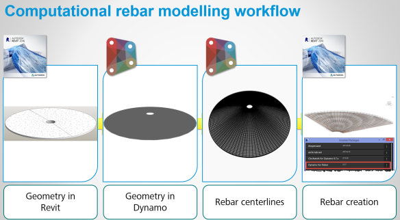
Revit geometry in Dynamo

To interpret the results better in Dynamo you’ll need the surrounding Revit geometry. This is done simultaneously with the large group of nodes at the bottom of the script.

Results

The final results look like this.

In Dynamo

In Revit

Special thanks to Nate Holland  and Andrew Heumann who were the initial “inspirators” for this.

Dataset

The Dynamo file and the “Sitting Man” family can be downloaded on this link.
As for the Revit file, you can simply use the “rac_advanced_sample_project.rvt” file from the Revit Sample Files.

Demo video

Radial Reinforcement in Revit with Dynamo

The modelling and detailing of reinforcement in a regular, circular floor in Revit can be done very straightforward using Path Reinforcement or by means of polar arrays.Once these circular floors have a varying thickness, and thus have a complex double curved top surface, the reinforcement modelling is best supported by using Dynamo.

In this post I will explain you how to introduce computational design for reinforcement modelling and this can be done in an easy way. At the end of the post you will be able to download the datasets and watch the instructional video.

Below you can see the circular shaped floor with an opening in the middle. The top surface of the floor has been edited with the “Modify Sub Elements” tool in Revit to get a varying thickness and to generate the double curvature of the face.

The goal is to model and detail the bottom (flat) and top (inclined) reinforcement in this floor.

With Dynamo, this whole process can be automated AND the equal rebars will be grouped in a rebar set, or the so called “Rebar Container”. By using a rebar container, the numbering and thus also the annotations can be set to a group of rebars, indicating the total amount of elements in the set of equal rebars.

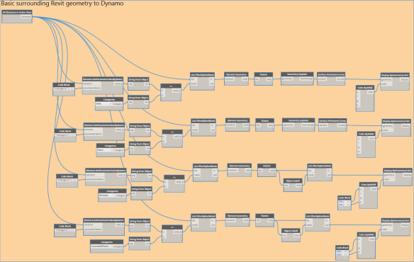
The applied workflow is practically the same for every “Dynamo rebar” project. You start by creating the appropriate geometry in Revit. Then you take the reference lines, faces or model in Dynamo. These references are then being used for the creation of the rebar centerlines. Therefore it is important that you re-calculate the cover from the formwork shape to the rebar centerlines by adding additional parameters (i.e. c1, c2, …like shown in the image below). Finally you create the rebar objects in the Revit model by using the “Dynamo for Rebar” package.

Datasets

The datasets that are used in the video below can be downloaded via this link.

Instructional video

If you want to learn how this is done, you can find the recorded screencast with voice-over on this link at Autodesk Knowledge Network (AKN).

Dynam(o)ite Your Design for Engineers @ AU 2015

Throughout this year I have been introducing carefully computational design with Dynamo in the world of the structural engineer. This by publishing posts on how to build up complex analysis models in Robot Structural Analysis and by reaching out to structural optimization techniques.

In one of my classes at Autodesk University 2015, I teached some of you how to actually apply these structural optimization techniques in Dynamo and Robot Structural Analysis. Although I find this a very advanced and heavy topic, still there was a great turnout at this class, which made me really happy !

Now the year is almost over, and it’s time for you to get up and running with these techniques. As promised I would share anything about this on this blog. Now is the time. You can find a full written step-by-step handout, the presentation and lots of datasets online now. Besides that, the class is recorded. So those who couldn’t make it to Las Vegas, watch the recording and learn about Dynamo and Optimo at your won pace.

Here’s the link to the class materials : 
 ES9542 – Dynam(o)ite Your Design for Engineers

Rebar modelling in Revit with Dynamo @ AU2015

In one of my classes at Autodesk University 2015, I presented a part about how to drive Structural Rebar in Revit, applying computational design techniques with Dynamo. The workflow I applied involved MS Excel, Revit and of course Dynamo.

I recorded a small video that illustrates this workflow:

If you want to learn this yourself, then you can rewatch the AU2015 class and download all the datasets and handout by clicking the link below:

MSF11845 – Dynam(o)ite Your Design from Concept to Fabrication

Rebar modelling in Revit with Dynamo for blended shapes

Since a few weeks, the package “Dynamo for Rebar” has been released. With this package, Dynamo allows you to model Rebar objects in Autodesk Revit. This opens up a lot of opportunities for automating rebar generation, complex shape modelling and so on…

In this topic I want to explain you more about a script I made in Dynamo to generate a steel rebar cage in a blend-shaped concrete column.

    

There are a few conditions which the rebar objects need to meet in this design:

• The longitudinal bars need to follow the inclination of the blended shape
• The hooks at the bottom of the longitudinal rebar will different for each bar that has another inclination
• The hooks need to point to the center of the bottom face of the column.
• The stirrups vary in size depending on their relative height position in the column (that’s an obvious one)

    

The datasets can be downloaded here. This script is working in Revit 2016, Dynamo 0.8.2 and the package Dynamo for Rebar v1.7.

The video below shows how the script works. You will find out that it is pretty handy to use. You can also apply this script to beams with varying height, though the longitudinal rebar might be changed a bit in Dynamo to get rid of the special hooks.

If you want to see more of this into depth, then register for one of my classes on Dynamo at Autodesk University 2015 in Las Vegas:

MSF11845 – Dynam(o)ite Your Design from Concept to Fabrication
Monday, Nov 30, 2:45 PM – 3:45 PM  (Fabrication Forum)

Animated effects of time dependant harmonic loads on a building

Today, I had a very deep dive into Robot Structural Analysis, when teaching the Northern European channel partners. At a certain moment David Truyens from Datech Belgium came up with a funny video of one guy trashing his washing machine by putting bricks in it. In fact the brick causes a heavy unbalance of the machine, with disastrous consequences. Have a look at it yourself on this link. Notice the wooden pallet that supports the machine.

So I started thinking how this would look like on a building structure, supporting this washing machine, or something simular poking the floors of the building. I ended up building up a Time History Analysis in Autodesk Robot Structural Analysis.

The video below shows you the steps to take in order to make an animated result of the effect of a time dependant, harmonic load on the structure. The simulation is done by applying a horizontal force with a sine function over a defined time period for a frequency of 3Hz and analogue a vertical force applied with a cosine function.

Tip: While watching the last 20 seconds of the video you could listen to some music like the “Harlem shake”.